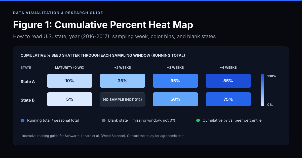
The search phrase “Figure 1 heat map indicating the cumulative percent” comes from an agricultural weed-science figure on seed shatter around soybean harvest, not a financial market map. Specifically, Figure 1 maps the cumulative percent of total seasonal weed seed production that had already shattered (fallen from the plant) across participating U.S. states in 2016 and 2017, measured at soybean physiological maturity and during the weeks that followed.
Quick answer (30-second takeaway):
- What color shows: Darker or higher-bin colors mean a larger cumulative percentage of the entire season’s weed seed production had already fallen to the ground by that sampling window.
- What cumulative percent means: It is a running total through that week divided by total seasonal seed production, not the percentage that fell during that single week alone.
- What a blank state means: A blank or unshaded state had no qualifying sample in that time window. It does not mean 0% seed shatter.
- What it is not: Cumulative percent (part of a whole accumulated over time) is not the same as percentile rank (standing relative to peers, such as on a stock heat map).
Exact Figure 1 caption and study context
If you encountered the prompt “Figure 1 heat map indicating the cumulative percent” in a biology, agronomy, data-literacy, or research-methods assignment, it refers to Figure 1 from the multi-state Weed Science study by Lauren M. Schwartz-Lazaro and colleagues:
- Part 2 (Grass species): “Seed-shattering phenology at soybean harvest of economically important weeds in multiple regions of the United States. Part 2: Grass species” (Weed Science, Cambridge University Press).
- Part 1 (Broadleaf species): Companion paper applying the same cumulative seed-shatter methodology to major broadleaf weeds such as Palmer amaranth, waterhemp, common lambsquarters, and giant ragweed.
In the published figure caption, Figure 1 is described as a heat map indicating the cumulative percent of seed shatter across grass species (such as barnyardgrass, giant foxtail, shattercane, and johnsongrass) by U.S. state in 2016 and 2017, evaluated at soybean maturity, 2 weeks after maturity, 3 weeks after maturity, and 4 weeks after maturity. Crucially, the caption notes that states were plotted in a given panel only when sampling occurred within that specific time window.
Why did the researchers build this heat map? Because harvest weed seed control (HWSC) methods, such as impact mills or chaff collection at combine harvest, only destroy weed seeds that are still attached to the plant when soybeans are harvested. If Figure 1 shows a high cumulative percent of seed shatter before or shortly after soybean maturity, most of those weed seeds are already on the soil surface and cannot be captured by delaying harvest.
The figure organizes four variables at once:
| Dimension in Figure 1 |
What it represents |
How to read it |
| U.S. state |
Participating state where weed plants were monitored |
Compare regional timing only when both states have data in the same panel |
| Year (2016 vs. 2017) |
Separate annual columns/panels |
Check whether rapid or slow shattering repeated across growing seasons |
| Sampling window |
Soybean maturity (0 wk), +2 wk, +3 wk, +4 wk |
Aligned to crop biological stage, not a single calendar date |
| Heat map color bin |
Cumulative percent of seasonal seed production shattered (0% to 100%) |
Higher bins mean less seed remains on the plant for harvest capture |
How Figure 1 heat map indicating the cumulative percent is calculated
In statistics and data visualization, cumulative percent means the running total up to a specific point, expressed as a percentage of the final total. It never measures a single isolated interval in a vacuum.
In the Weed Science seed-shattering studies, the formula for each observation window is:
Cumulative Percent Seed Shatter = 100 × (Seeds shattered from start of monitoring through current week ÷ Total seasonal seed production)
Where total seasonal seed production equals:
- All seeds captured in seed traps during weekly field sampling windows, plus
- All seeds still retained on the maternal plant heads/panicles at final harvest collection.
Worked numerical example
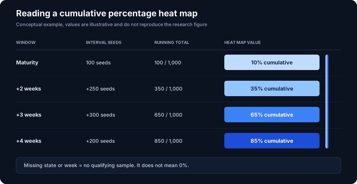
Suppose a monitored weed population in one state produced 1,000 total seeds over the season:
| Sampling window |
Seeds shattered in this interval alone |
Running shattered total (cumulative) |
Value shown on Figure 1 heat map |
Seed still retained on plant |
| Soybean maturity |
100 |
100 / 1,000 |
10% |
900 (90%) |
| Maturity + 2 weeks |
250 |
350 / 1,000 |
35% |
650 (65%) |
| Maturity + 3 weeks |
300 |
650 / 1,000 |
65% |
350 (35%) |
| Maturity + 4 weeks |
200 |
850 / 1,000 |
85% |
150 (15%) |
Notice how to interpret the 65% cell at Maturity + 3 weeks:
- Correct interpretation: By three weeks after soybean maturity, 65% of the entire season’s seeds (650 of 1,000) had already fallen off the plants, leaving only 35% available for harvest weed seed control.
- Wrong interpretation: It does not mean 65% of the seeds fell during week 3 alone (only 300 seeds, or 30% of the seasonal total, fell between week 2 and week 3).
Because cumulative percentage is a non-decreasing running share of the seasonal total, a state’s cumulative value across sequential panels for the same population stays flat or increases from maturity toward +4 weeks.
How to read Figure 1 step by step
1. Separate 2016 and 2017 before drawing conclusions
Start by scanning down a single year column (2016 first, then 2017). Heat maps make cross-panel comparisons look effortless, but year-to-year differences can reflect rainfall, temperature, soybean cultivar maturity, or which specific states sampled in each window. When a state shifts into dark/high-shatter color bins early in both 2016 and 2017, the biological pattern is much stronger.
2. Anchor on biological time (soybean maturity), not calendar month
Soybeans reach physiological maturity at different calendar dates in Arkansas, Missouri, Indiana, or Wisconsin. Figure 1 standardizes time around soybean maturity so that “2 weeks after maturity” compares weeds at the same stage of crop harvest readiness across latitudes.
3. Map the color shade to the legend’s percentage range
Heat maps group continuous numbers into visual gradients or discrete color steps. Always check the color bar before claiming two states had identical shatter rates. Two states with similar mid-tone shading may sit several percentage points apart within the same legend band.
4. Track the slope of change across weeks
The practical story in Figure 1 is how fast the map darkens:
- High percentage already at maturity: Substantial seed loss happened before soybeans were even ready to harvest.
- Steep jump between maturity and +2 or +3 weeks: Every week of harvest delay returns a large fraction of weed seed to the soil seedbank.
- Low cumulative percentage through +3 or +4 weeks: Most seeds stayed on the plant, making harvest weed seed destruction highly effective.
5. Read blank or uncolored states as “no sample in window,” never “0%”
This is the #1 test-question and peer-review trap on Figure 1. When a state is unshaded or absent in a specific panel, it had no qualifying field sample during that standardized time window.
A blank state does not indicate:
- 0% weed seed shatter,
- absence of grass weeds in that state, or
- superior weed management.
Why some states appear in one week and disappear in another
In multi-state field agronomy, researchers cannot always visit every site on the exact day soybeans hit maturity plus 14, 21, or 28 days. Weather delays, wet fields, and regional scheduling create uneven sampling dates.
The study authors explicitly cite Arkansas in 2017 to illustrate their rule: field collection dates in Arkansas did not fall inside the strict cutoff for the maturity window or the maturity + 2-week window, so Arkansas is left blank in those panels and appears in the maturity + 3-week panel where the sample date matched the protocol.
Leaving unmatched windows blank preserves scientific honesty. Interpolating or copying an out-of-window number would create a fuller-looking map while corrupting the biological timeline. Buydy applies the exact same missing-data discipline on our stock heat map and ETF heat map: when an issuer or fund lacks valid underlying data for a metric, the cell remains a dash (-) rather than receiving a fabricated fallback score.
Cumulative percent vs. percentage change vs. percentile rank
Many students and analysts lose points, or misread research dashboards, because three percentage terms look nearly identical in a heat map legend. Here is the exact distinction:
| Metric type |
Formula / definition |
Range & direction |
Example in practice |
| Cumulative percent (Figure 1) |
100 × running total through time t ÷ final total |
0% to 100%; monotonically non-decreasing over time |
65% of seasonal weed seeds had shattered by 3 weeks after soybean maturity |
| Interval percent / share |
100 × amount in interval t ÷ final total |
0% to 100%; can rise or fall each week; sums to 100% across all intervals |
30% of total seasonal seeds shattered specifically between week 2 and week 3 |
| Percentile rank (Buydy heat maps) |
Peer ranking from 0th to 100th within a defined comparison group |
0 to 100 at a single snapshot; changes when peers change |
A stock sits in the 65th percentile for dividend growth within its sector |
If you are transitioning from academic heat maps to financial analysis, see our complete guide on how to read a stock heat map for how peer percentiles work alongside raw values.
Common mistakes when interpreting Figure 1 (and how to avoid them)
- Treating weekly panels as independent weekly losses. If Maturity is 15% and +2 Weeks is 45%, the additional shatter during those two weeks was 30 percentage points, not 45%.
- Assuming geography alone caused the color differences. Figure 1 pools grass weed observations at the state level. Differences between states reflect a mix of grass species composition, local biotypes, temperature, rainfall, and maturity dates, not latitude by itself.
- Comparing states across different time rows. Comparing State A at Maturity to State B at +4 Weeks mixes two different stages of crop senescence. Compare states within the same time window, or compare one state across time.
- Treating missing panels as zero shatter. Always verify whether a state was sampled in that window before citing it as a low-shatter region.
7-point checklist for reading any cumulative percentage heat map
Whether you are grading an agronomy paper, reviewing an epidemiology curve, or auditing a financial cohort table, run this checklist before trusting the colors:
- What is being accumulated? (Weed seeds, cumulative revenue, cohort defaults, rainfall?)
- What is the denominator? (Total seasonal production per plant, initial cohort size, or annual quota?)
- What is the time zero anchor? (Calendar date, soybean physiological maturity, or product launch?)
- Are color bands continuous or binned? (Check the legend breaks before estimating exact numbers.)
- How are missing observations encoded? (Gray, white, dashed, or omitted?)
- Can the curve ever decrease? (True cumulative shares of a fixed positive total should not drop; if a panel drops, the sample composition changed.)
- Where are the raw numbers? (Use the heat map to spot the pattern, then check the underlying table or model before making a decision.)
In investment research, pairing visual color scans with raw numbers and strict missing-data rules prevents false confidence. You can see how that workflow operates across equities and funds in stock heat map vs stock screener and on our research resources hub.
Sources and references
This educational guide explains how to read and interpret the published figure and methodology; it does not reproduce copyrighted journal imagery. The diagram on this page uses illustrative values to teach the cumulative calculation.
- Schwartz-Lazaro, L. M., et al. (2021). Seed-shattering phenology at soybean harvest of economically important weeds in multiple regions of the United States. Part 2: Grass species. Weed Science, 69(1), 104-110. https://doi.org/10.1017/wsc.2020.79
- Schwartz-Lazaro, L. M., et al. (2021). Seed-shattering phenology at soybean harvest of economically important weeds in multiple regions of the United States. Part 1: Broadleaf species. Weed Science, 69(1), 95-103. https://doi.org/10.1017/wsc.2020.80
- Zenodo figure record: Figure 1 heat map indicating the cumulative percent of seed shatter. https://doi.org/10.5281/zenodo.12534076
FAQ
What does the Figure 1 heat map indicating the cumulative percent show?
It shows the cumulative percentage of total seasonal weed seed production that had already shattered (fallen from the plant) across participating U.S. states in 2016 and 2017, measured at soybean maturity and 2, 3, and 4 weeks after maturity.
How is cumulative percent calculated in Figure 1?
Cumulative percent is calculated as 100 × (seeds shattered through that sampling window ÷ total seasonal seed production), where total seasonal production is all shattered seeds collected in traps plus seeds remaining on the plant at final harvest.
Why are some states blank or missing in certain weeks on Figure 1?
A state is only colored in a panel when field sampling took place within that specific time window (for example, soybean maturity or maturity + 2 weeks). A blank state means no qualifying sample was collected in that window, not that seed shatter was 0%.
What does a darker or higher-percentage color mean for weed management?
A higher cumulative percentage means most of the weed’s seasonal seeds have already fallen to the ground before or during harvest delay, leaving fewer seeds on the plant where harvest weed seed control (HWSC) tools can capture and destroy them.
Why does cumulative percent increase from maturity to 4 weeks after maturity?
Because each later window is a running total that includes all seeds shattered in earlier windows plus any new seeds that shattered since the prior sample.
What is the difference between cumulative percent and percentile rank on a heat map?
Cumulative percent measures how much of a single total has accumulated up to a point in time (0% to 100% of total seed production). Percentile rank measures how one item ranks against a peer group at a given moment (such as ranking a company in the 80th percentile of its sector).
Continue learning
Research education only. Always consult the original Weed Science papers for agronomic data and scientific conclusions.